CGVB for Bayesian Logistic Regression model object

CGVB for Bayesian Logistic Regression model Github code

This example implements the example 3.4 shown in the VB tutorial paper.

Load the LabourForce data as a matrix. The last column is the response variable.

% Random seed to reproduce results 
rng(2020)

% Load the LabourForce dataset
labour = readData('LabourForce',...
                  'Type','Matrix',...
                  'Intercept',true);

Create a LogisticRegression model object by specifying the number of parameters as the input argument. Use normal distribution with zero mean and $50$ variance priors for model coefficients.

% Number of input features
n_features = size(labour,2)-1;
% Define a LogisticRegression model object
Mdl = LogisticRegression(n_features,...
                         'Prior',{'Normal',[0,50]});

Run CGVB to obtain VB approximation of the posterior distribution of model parameters. By default, the algorithm will initialize the variational parameters using a normal distribution with a small variance.

%% Run Cholesky GVB with random initialization
Estmdl_1  = CGVB(Mdl,labour,...
                'LearningRate',0.002,...  % Learning rate
                'NumSample',50,...        % Number of samples to estimate gradient of lowerbound
                'MaxPatience',20,...      % For Early stopping
                'MaxIter',5000,...        % Maximum number of iterations
                'GradWeight1',0.9,...     % Momentum weight 1
                'GradWeight2',0.9,...     % Momentum weight 2
                'WindowSize',10,...       % Smoothing window for lowerbound
                'StepAdaptive',500,...    % For adaptive learning rate
                'GradientMax',10,...      % For gradient clipping    
                'LBPlot',false);          % Dont plot the lowerbound when finish

Or we can manually specify initial values for variational mean. A convenient choice is to use MLE estimation of model parameters, if available.

%% Run Cholesky GVB with MLE initialization
% Random seed to reproduce results 
rng(2020)

theta_init = Mdl.initParams('MLE',labour); 
Estmdl_2  = CGVB(Mdl,labour,...
                'MeanInit',theta_init,... % Initial values of variational mean
                'LearningRate',0.002,...  % Learning rate
                'NumSample',50,...        % Number of samples to estimate gradient of lowerbound
                'MaxPatience',20,...      % For Early stopping
                'MaxIter',5000,...        % Maximum number of iterations
                'GradWeight1',0.9,...     % Momentum weight 1
                'GradWeight2',0.9,...     % Momentum weight 2
                'WindowSize',10,...       % Smoothing window for lowerbound
                'StepAdaptive',500,...    % For adaptive learning rate
                'GradientMax',10,...      % For gradient clipping    
                'LBPlot',false);          % Dont plot the lowerbound when finish

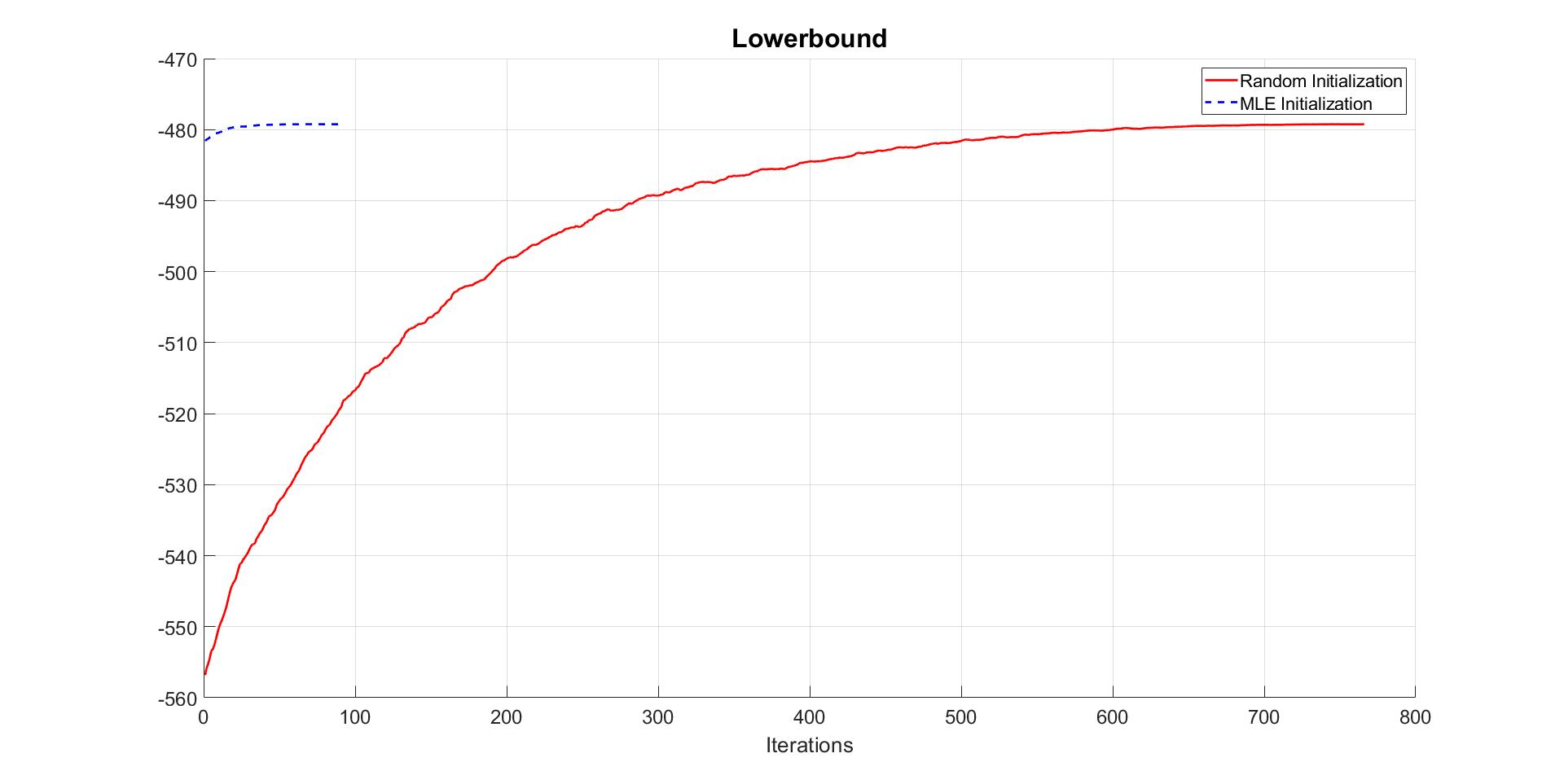
We then can compare the covergence of the lowerbound in two cases.

% Compare convergence of lowerbound in 2 cases 
figure
hold on
grid on
plot(Estmdl_1.Post.LB_smooth,'-r','LineWidth',2)
plot(Estmdl_2.Post.LB_smooth,'--b','LineWidth',2)
title('Lowerbound')
legend('Random Initialization','MLE Initialization' )

The plot of lowerbound shows that the CGVB algorithm converges well. The algorithm converges much faster when we use MLE estimates as starting points. This example shows that choosing initial values for variational parameters is very important for VB methods in general.

We can check how close the variational distribution is to the true posterior densities of model paramters. We run MCMC to obtain samples of model parameters from their posterior distribution.

% It is useful to compare the approximate posterior density to the true density obtain by MCMC
Post_MCMC = MCMC(Mdl,labour,...
                 'NumMCMC',50000,...         % Number of MCMC iterations
                 'ParamsInit',theta_init,... % Using MLE estimates as initial values
                 'Verbose',100);             % Display sampling information after each 100 iterations

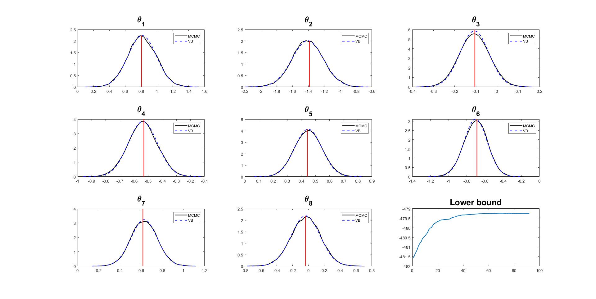
Given the MCMC samples of the posterior density of model paramters, we can compare the true and approximate posterior distribution.

% Compare densities by CGVB and MCMC
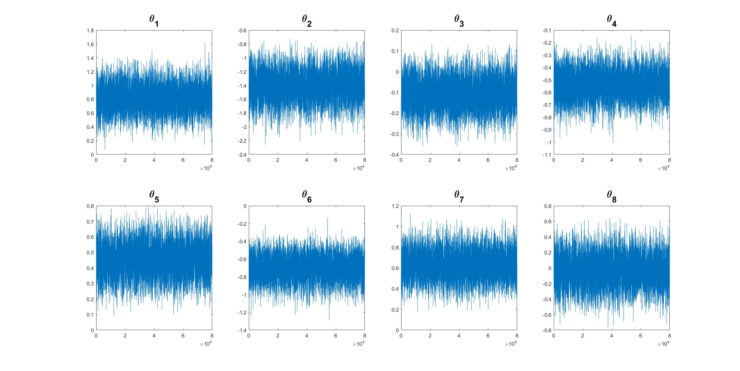
% Get posterior mean and trace plot for a parameter to check the mixing 
[mcmc_mean,mcmc_std,mcmc_chain] = Post_MCMC.getParamsMean('BurnInRate',0.2,...         % Throw away 20% samples
                                                          'PlotTrace',1:n_features,... % Trace plot for all parameters
                                                          'SubPlot',[2,4]);            % Dimension of subplots

% Plot density
fontsize  = 20;
numparams = Estmdl_2.Model.NumParams;

% Extract variation mean and variance
mu_vb     = Estmdl_2.Post.mu;
sigma2_vb = Estmdl_2.Post.sigma2;

figure
for i = 1:numparams
    subplot(3,3,i)
    xx = mcmc_mean(i)-4*mcmc_std(i):0.002:mcmc_mean(i)+4*mcmc_std(i);
    yy_mcmc = ksdensity(mcmc_chain(:,i),xx,'Bandwidth',0.022);  
    yy_vb = normpdf(xx,mu_vb(i),sqrt(sigma2_vb(i)));    
    plot(xx,yy_mcmc,'-k',xx,yy_vb,'--b','LineWidth',1.5)
    line([theta_init(i) theta_init(i)],ylim,'LineWidth',1.5,'Color','r')    
    str = ['\theta_', num2str(i)];   
    title(str,'FontSize', fontsize)
    legend('MCMC','VB')
end
subplot(3,3,9)
plot(Estmdl_2.Post.LB_smooth,'LineWidth',1.5)
title('Lower bound','FontSize', fontsize)

The trace plots of MCMC samples of model parameters shows that the MCMC algorithm works properly.

The plots of variational densities and true posterior densities show that the CGVB algorithm works efficiently in this example.