VBLab Custom Model

VBLab provides several ways for custom-built models that work with VB algorithm classes such as CGVB, VAFC, MGVB and NAGVAC.

Define custom models as function handles

The supported VB algorithms take statistical models and training data as inputs in order to compute the $\nabla_\theta h(\theta)$ and $h(\theta)$ terms. This model- and data-specific information can be provided to the VB algorithms as a function handle with some rules. The following template is suggested when users define their statistical models as functions to compute the $\nabla_\theta h(\theta)$ and $h(\theta)$ terms in each iteration of the CGVB, VAFC and NAGVAC algorithms.

function [h_func_grad,h_func] = grad_h_func(data,theta,setting)
end

For the MGVB algorithm, users only need to define the function to compute the $h(\theta)$ term and the following template is suggested

function h_func = h_func(data,theta,setting)
end

It is not required to use exactly the same name for function and input/output arguments but the input and outputs arguments have to be defined exactly in the same order. Descriptions for input and output arguments are as follows

Input	Description
`data`	• The training data. Denote as $y$ in VB algorithms. • This is also the `data` arguments when calling VB classes such as CGVB, VAFC, MGVB and NAGVAC.
`theta`	• A column vector of model parameters in each VB iteration. Denote as $\theta$ in VB algorithms. • For GVB, $\theta$ is generated from a multivariate normal distribution. Then if $\theta$ is restricted, e.g. prior distribution is not normal, then a transformation of $\theta$ to original scale, together with the jacobian, have to be provided.
`setting`	• Additional settings of the custom models. • For example, prior distribution or some constant terms to define the models.
`h_func_grad`	• Gradient vector $\nabla_\theta h(\theta) = \nabla_\theta \text{log}p(y \mid \theta) + \nabla_\theta \text{log} p(\theta)$. • Must be a column vector $1 \times D$ with $D$ the number of model parameters.
`h_func`	• $h(\theta) = \text{log} p(y \mid \theta) + \text{log} p(\theta)$. • Must be a scalar.

Note:

If the statistical models are defined as function handles, users have to specify the number of model parameters explicitly using the 'NumParams' argument of VB classes.
This approach is more suitable for simple models. For complicated models, it is advisable to define custom models as Matlab classes, which will be discussed in the next section.

Example: Define a Logistic Regression model as a function handle. Github code

This example shows how to define a Logistic Regression model as function handles to run with the CGVB, VAFC and NAGVAC algorithms. See mathematical derivation of the $\nabla_\theta h(\theta)$ and $h(\theta)$ terms of Logistic Regression model in the tutorial example 3.4.

First, load the LabourForce data as a matrix. The last column is the response variable.

% Load the LabourForce dataset
labour = readData('LabourForce',...
                  'Type','Matrix',...
                  'Intercept',true);

Prepare some variables needed to run the VB algorithm and to define the custom model.

% Number of input features
n_features = size(labour,2)-1;
setting.Prior = [0,50];

In this example, we use the CGVB technique to fit the custom model on the labour data. To run the CGVB technique with the custom model, we need to specify the handle of the function defining the custom model as the first input argument. We also need to explicitly provide the number of model parameters for the 'NumParams' argument. Finally, we need to pass additional information, e.g. priors, stored in the struct setting to the 'Setting' argument. This setting variable then will be passed to the custom function as the input argument.

% Run CGVB to obtain VB approximation of the posterior distribution
Post = CGVB(@grad_h_func_logistics,...  % Function handle to define the custom model
            labour,...                  % Training data    
            'NumParams',num_feature,... % Number of model parameters
            'Setting',setting,...       % Additional setting of the custom models
            'LearningRate',0.002,...    % Learning rate
            'NumSample',50,...          % Number of samples to estimate gradient of lowerbound
            'MaxPatience',20,...        % For Early stopping
            'MaxIter',5000,...          % Maximum number of iterations
            'InitMethod','Random',...   % Randomly initialize variational mean
            'GradWeight1',0.9,...       % Momentum weight 1
            'GradWeight2',0.9,...       % Momentum weight 2
            'WindowSize',10,...         % Smoothing window for lowerbound
            'GradientMax',10,...        % For gradient clipping
            'LBPlot',true);             % Plot the lowerbound when finish

The output Post is a struct storing information about estimation results and the VB algorithm. See the output of CGVB, VAFC, MGVB and NAGVAC for more details.

We then define the function grad_h_func_logistics to compute the $\nabla_\theta h(\theta)$ and $h(\theta)$ terms using their mathematical derivation shown in the tutorial example 3.4.

% Define gradient of h function for Logistic regression 
% theta: Dx1 array
% h_func: scalar
% h_func_grad: Dx1 array
function [h_func_grad,h_func] = grad_h_func_logistics(data,theta,setting)

    % Extract additional settings
    d = length(theta);
    sigma2 = setting.Prior(2);
    
    % Extract data
    X = data(:,1:end-1);
    y = data(:,end));
    
    % Compute log likelihood
    aux = X*theta;
    llh = y.*aux-log(1+exp(aux));
    llh = sum(llh);  
    
    % Compute gradient of log likelihood
    ppi       = 1./(1+exp(-aux));
    llh_grad  = X'*(y-ppi);

    % Compute log prior
    log_prior =-d/2*log(2*pi)-d/2*log(sigma2)-theta'*theta/sigma2/2;
    
    % Compute gradient of log prior
    log_prior_grad = -theta/sigma2;
    
    % Compute h(theta) = log p(y|theta) + log p(theta). Must be a scalar
    h_func = llh + log_prior;
    
    % Compute gradient of the h(theta)
    h_func_grad = llh_grad + log_prior_grad;

    % h_func_grad must be a Dx1 column
    h_func_grad = reshape(h_func_grad,length(h_func_grad),1);
end    

Note:

The grad_h_func_logistics() function can be defined in a separated Matlab script named grad_h_func_logistics.m or defined in the same script running the example. For the latter case, the function has to be defined at the end of the script.
In some cases, deriving the gradient $\nabla_\theta h(\theta)$ can be troublesome. We can compute it using Matlab’s Automatic Differentiation facility, which is a technique for evaluating derivatives numerically and automatically. See Matlab Automatic Differentiation tutorials. See example define a Logistic Regression model as function handle using Matlab AutoDiff

Define custom models as Matlab Class Objects

For complicated models, it is more efficient to define the models as Matlab classes as the model-specific information can be conveniently stored in classes’ properties and methods. The following template is the minimum requirement to define the custom models as Matlab classes:

classdef CustomModel
    
    % Define model-specific properties
    properties
        ModelName      % Model name 
        NumParams      % Number of parameters
        Post           % Struct to store training results (maybe not used)   
    end
    
    % Define model-specific methods
    methods
        % Constructor. This will be automatically called when users create a CustomModel object
        function obj = CustomModel(inputArg1,inputArg2)
            % Set value for ModelName and NumParams
            ModelName = ...
            NumParams = ...
        end
        
        % Function to compute gradient of h_theta and h_theta
        % For CGVB, VAFC, NAGVAC
        function [h_func_grad, h_func] = hFunctionGrad(obj,data,theta)
        end  

        % Function to compute h_theta
        % For MGVB
        function h_func = hFunction(obj,data,theta)
        end  
    end
end

The two following properties have to be defined and assigned values within the constructor.

`ModelName`	string	Name of the custom model
`NumParams`	Integer	Number of model parameters

In general, the hFunctionGrad() and hFunction() methods are defined in the same way and play the same role as the corresponding functions discussed in the previous section. However, there are two main differences between two approaches:

First, users have to name the methods to compute the $\nabla_\theta h(\theta)$ and $h(\theta)$ terms exactly as hFunctionGrad and hFunction while the class name and hence the class constructor name can be defined arbitrarily.
- The VB classes such as VAFC, NAGVAC, CGVB then will call the hFunctionGrad method of the provided model object in each VB iteration to compute the $\nabla_\theta h(\theta)$ and $h(\theta)$ terms.
- Similarly, the MGVB class will call the hFunction method of the provided model object in each VB iteration to compute the $h(\theta)$ term.
Second, users can store additional information about the model in class properties and methods and hence don’t need to use a struct to do the same task as discussed in the previous section.

For example, the VB classes such as CGVB, VAFC and NAGVAC will run the following code to compute the $\nabla_\theta h(\theta)$ and $h(\theta)$ terms of the provided model.

[grad_h_theta,h_theta] = model.hFunctionGrad(data,theta); 

Example: Define a VAR(1) model as a Matlab class. Github code

This example shows how to define a VAR(1) model using Matlab class and fit the model on a simulation data using CGVB algorithm. For the detailed discussion of mathematical derivations and model properties, see the example of how to define a VAR(1) model as a function handle. We use standard normal distribution for the priors and a constant covariance matrix.

First, we define the VAR1 class in a separated script named VAR1.m. See the Matlab code of the VAR1 class defined in this example here.

classdef VAR1
    %VAR1 Class to model the VAR(1) model
    
    properties 
        ModelName      % Model name 
        NumParams      % Number of parameters
        Prior          % Prior object
        ParamIdx       % Indexes of model parameters in the vector of variational parameters
        Gamma          % Fix covarian matrix
    end
    
    methods
        % Constructor. This will be automatically called when users create a VAR1 object
        function obj = VAR1(NumSeries)
            % Set value for ModelName and NumParams
            obj.ModelName  = 'VAR1';                 
            obj.NumParams  = NumSeries + NumSeries^2; 
            obj.Prior      = [0,1]; % Use a normal distribution for prior
            obj.ParamIdx.c = 1:NumSeries;
            obj.ParamIdx.A = NumSeries+1:obj.NumParams;
            obj.Gamma      =  0.1*eye(NumSeries);
        end
        
        % Function to compute gradient of h_theta and h_theta
        function [h_func_grad, h_func] = hFunctionGrad(obj,y,theta)
            % Extract size of data
            [m,T] = size(y);
                
            % Extract model properties
            prior_params = obj.Prior;
            d = obj.NumParams;
            idx = obj.ParamIdx;
            gamma = obj.Gamma;
            gamma_inv = gamma^(-1);

            % Extract params from theta
            c = theta(idx.c);                               % c is a column
            A = reshape(theta(idx.A),length(c),length(c));  % A is a matrix
                
            % Log prior
            log_prior = Normal.logPdfFnc(theta,prior_params);
                
            % Log likelihood
            log_llh = 0;
            for t=2:T
                log_llh = log_llh -0.5*(y(:,t) - A*y(:,t-1)-c)' * gamma_inv * (y(:,t) - A*y(:,t-1)-c);
            end  
            log_llh = log_llh - 0.5*m*(T-1)*log(2*pi) - 0.5*(T-1)*log(det(gamma));

            % Compute h_theta
            h_func = log_prior + log_llh;
                
            % Gradient log_prior
            grad_log_prior = Normal.GradlogPdfFnc(theta,prior_params);
                
            % Gradient log_llh;
            grad_llh_c = 0;
            grad_llh_A = 0;
            for t=2:T
                grad_llh_c = grad_llh_c + gamma_inv*(y(:,t) - A*y(:,t-1)-c);
                grad_llh_A = grad_llh_A + kron(y(:,t-1),gamma_inv*(y(:,t) - A*y(:,t-1)-c));
            end
                
            grad_llh = [grad_llh_c;grad_llh_A(:)];
                
            % Compute Gradient of h_theta
            h_func_grad = grad_log_prior + grad_llh;
            
            % Make sure grad_h_theta is a column
            h_func_grad = reshape(h_func_grad,d,1);
        end  
    end
end

Given the class VAR1, we can run an example of fit the VAR(1) model on a simulation data using CGVB algorithm as following

% Setting
m = 2;   % Number of time series
T = 100; % Number of observations

% Generate simulation data
y = randn(m,T);

% Create a VAR1 model object
Mdl = VAR1(m);

%% Run CGVB to fit the VAR1 model object
Post_CGVB_VAR1 = CGVB(Mdl,y,...
                      'LearningRate',0.002,...       % Learning rate
                      'NumSample',50,...             % Number of samples to estimate gradient of lowerbound
                      'MaxPatience',20,...           % For Early stopping
                      'MaxIter',5000,...             % Maximum number of iterations
                      'GradWeight1',0.9,...          % Momentum 1
                      'GradWeight2',0.9,...          % Momentum 2
                      'WindowSize',10,...            % Smoothing window for lowerbound
                      'GradientMax',10,...           % For gradient clipping
                      'LBPlot',false); 

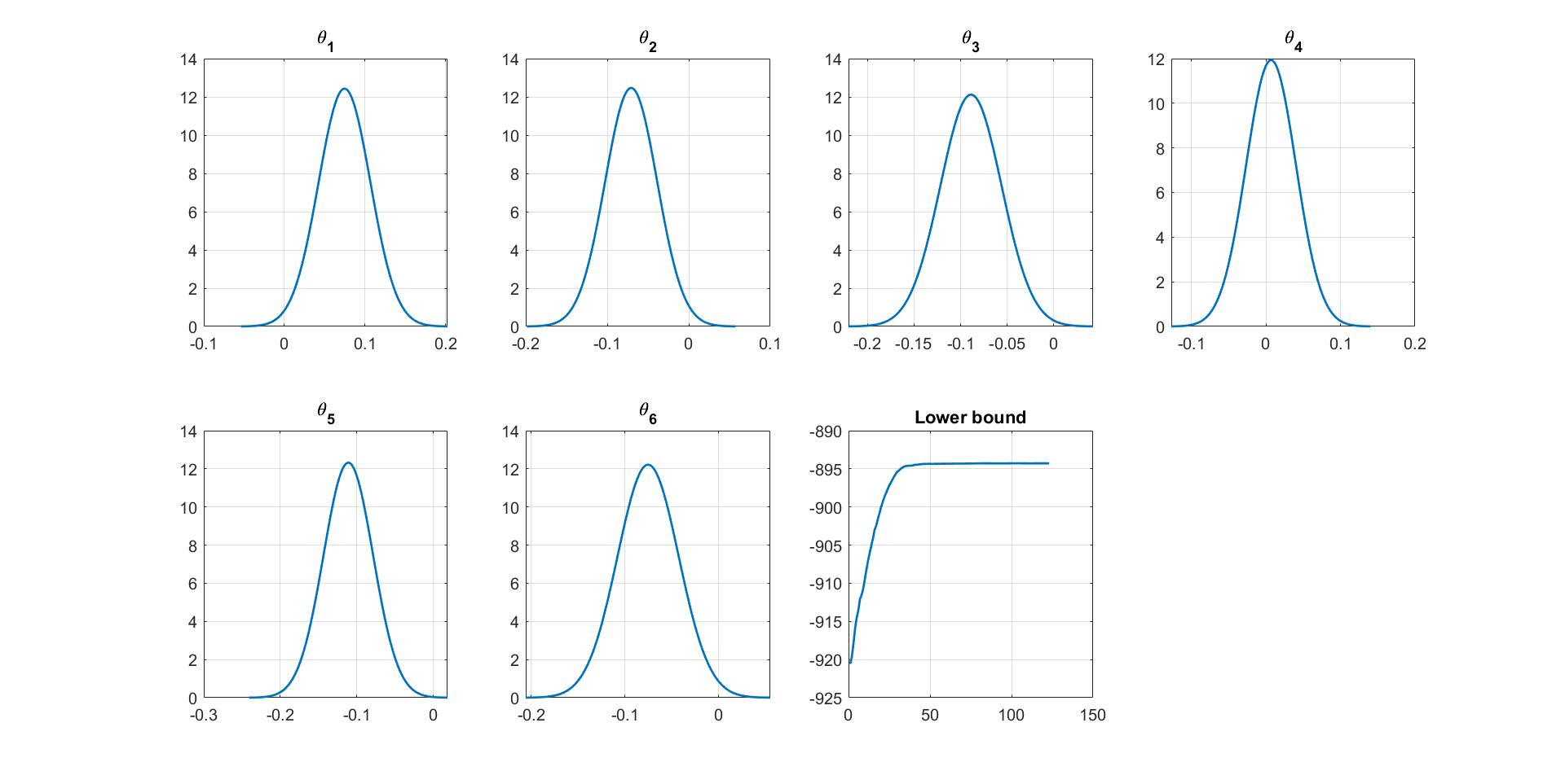
We can manually plot the variational distribution together with the lowerbound. The convergence of the lowerbound shows that the CGVB works properly in this example.

%% Plot variational distributions and lowerbound 
figure
% Extract variation mean and variance
mu_vb     = Post_CGVB_VAR1.Post.mu;
sigma2_vb = Post_CGVB_VAR1.Post.sigma2;

% Plot the variational distribution of each parameter
for i=1:Post_CGVB_VAR1.Model.NumParams
    subplot(2,4,i)
    vbayesPlot('Density',{'Normal',[mu_vb(i),sigma2_vb(i)]})
    grid on
    title(['\theta_',num2str(i)])
    set(gca,'FontSize',15)
end

% Plot the smoothed lower bound
subplot(2,4,7)
plot(Post_CGVB_VAR1.Post.LB_smooth,'LineWidth',2)
grid on
title('Lower bound')
set(gca,'FontSize',15)        