Tutorial examples

Examples to illustrate the VB algorithms discussed in the tutorial paper. The examples are numbered in the same order as presented in the VB tutorial paper

• Example 2.1: Mean Field Variational Bayes for Bayesian Linear Regression
• Example 3.1: Fixed From VB with control variates for Bayesian Linear Regression
• Example 3.2: Fixed From VB with control variates and natural gradient for Bayesian Linear Regression
• Example 3.3: Hybrid Fixed From VB for Bayesian Linear Regression
• Example 3.4: Cholesky GVB for Bayesian Logistic Regression

---

Example 2.1: Mean Field Variational Bayes for Bayesian Linear Regression

$\def\t{\theta} \def\LB{\text{LB}} \def\E{\mathbb{E}} \def\KL{\text{KL}} \newcommand{\wh}{\widehat} \newcommand{\wt}{\widetilde} \def\F{\cal{F}} \def\N{\cal{N}} \def\s{\sigma} \def\a{\alpha} \def\b{\beta} \def\l{\lambda} \newcommand{\eps}{\epsilon}$

From (7), the optimal VB posterior for $\s^2$ is

\[\begin{eqnarray} q(\s^2)&\propto&\exp\left(\E_{-\s^2}[\log p( y,\mu,\s^2)]\right)=\exp\left(\E_{q(\mu)}[\log p( y,\mu,\s^2)]\right)\\ &\propto&\exp\left( \E_{q(\mu)}\left[\log p(\s^2)+\log p( y \mid \mu,\s^2)\right] \right)\\ &\propto&\exp\left(-(\a_0+\frac n2+1)\log\s^2-\left(\b_0+\frac12\E_{q(\mu)}\left[ \sum(y_i-\mu)^2\right]\right)/\s^2\right). \end{eqnarray}\]

In the above derivation, we have ignored all the constants independent of $\sigma^2$ as they are unnecessary for identifying the distribution $q(\sigma^2)$. It follows that $q(\s^2)$ is inverse-Gamma with parameters \(\a_q=\a_0+\frac n2,\;\;\;\;\b_q=\b_0+\frac12\E_{q(\mu)}\left[\sum(y_i-\mu)^2\right].\) Computation of the expecation $\E_{q(\mu)}(\cdot)$ becomes clear shortly after $q(\mu)$ is identified. From (8), the optimal VB posterior for $\mu$ is

\[\begin{eqnarray} q(\mu)&\propto&\exp\left(\E_{q(\s^2)}[\log p(y,\mu,\s^2)]\right)\\ &\propto&\exp\left(\E_{q(\s^2)}[\log p(\mu)+\log p( y \mid \mu,\s^2)]\right)\\ &\propto&\exp\left(-\frac{1}{2\s_0^2}(\mu^2-2\mu_0\mu)-\frac n2\E_{q(\s^2)}[\frac{1}{\s^2}](-2\bar y\mu+\mu^2)\right)\\ &\propto&\exp\left(-\frac{1}{2}\underbrace{\left(\frac{1}{\s_0^2}+n\E_{q(\s^2)}[ \frac{1}{\s^2}]\right)}_{A}\mu^2+\mu\underbrace{\left(\frac{\mu_0}{\s_0^2}+n\bar y\E_{q(\s^2)}[ \frac{1}{\s^2}]\right)}_B\right)\\ &=&\exp\left(-\frac{1}{2}A\mu^2+B\mu\right)\\ &\propto&\exp\left(-\frac12\frac{(\mu-{B}/{A})^2}{1/A}\right). \end{eqnarray}\]

It follows that $q(\mu)$ is Gaussian with mean $\mu_q$ and variance $\s_q^2$

\[\mu_q=\frac{\frac{\mu_0}{\s_0^2}+n\bar y\E_{q(\s^2)}[\frac{1}{\s^2}]}{\frac{1}{\s_0^2}+n\E_{q(\s^2)}[\frac{1}{\s^2}]},\;\;\;\;\; \s_q^2=\Big(\frac{1}{\s_0^2}+n\E_{q(\s^2)}[\frac{1}{\s^2}]\Big)^{-1}.\]

With the distributions $q(\mu)$ and $q(\sigma^2)$ having identified, we are now able to compute the expectations w.r.t. $q(\mu)$ and $q(\sigma^2)$ in the above:

\[\begin{eqnarray} \b_q&=&\b_0+\frac12\E_{q(\mu)}\left[\sum(y_i-\mu)^2\right]\\ &=&\b_0+\frac12\left(\sum y_i^2-2n\bar y\E_{q(\mu)}[\mu]+n\E_{q(\mu)}[\mu^2]\right)\\ &=&\b_0+\frac12\sum y_i^2-n\bar y\mu_q+\frac{n}{2}(\mu_q^2+\s_q^2). \end{eqnarray}\]

As $q(\s^2)\sim\text{Inverse-Gamma}(\a_q,\b_q)$, $\E(1/\s^2)=\a_q/\b_q$. Hence,

\[\mu_q=\Big(\frac{\mu_0}{\s_0^2}+n\bar y\frac{\a_q}{\b_q}\Big)/\Big(\frac{1}{\s_0^2}+n\frac{\a_q}{\b_q}\Big),\;\;\text{ and }\;\;\s_q^2=\Big(\frac{1}{\s_0^2}+n\frac{\a_q}{\b_q}\Big)^{-1}.\]

Note that we did not make any assumption on the parametric form of optimal variational distributions $q(\mu)$ and $q(\sigma^2)$, it is the model (the prior and the likelihood) that determines their form.

We arrive at the following updating procedure:

• Initialize $\mu_q,\s_q^2$
• Update the following recursively

\[\begin{eqnarray} \a_q&\leftarrow&\a_0+\frac n2,\\ \b_q&\leftarrow&\b_0+\frac12\sum y_i^2-n\bar y\mu_q+\frac{n}{2}(\mu_q^2+\s_q^2),\\ \mu_q&\leftarrow&\Big(\frac{\mu_0}{\s_0^2}+n\bar y\frac{\a_q}{\b_q}\Big)/\Big(\frac{1}{\s_0^2}+n\frac{\a_q}{\b_q}\Big),\\ \s_q^2&\leftarrow&\Big(\frac{1}{\s_0^2}+n\frac{\a_q}{\b_q}\Big)^{-1}, \end{eqnarray}\]

until convergence

We can stop the iterative scheme when the change of the $\ell_2$-norm of the vector $\l=(\a_q,\b_q,\mu_q,\s_q^2)^\top$ is smaller than some $\eps$, $\eps=10^{-5}$ for example. We can also initialize $\a_q,\b_q$ and then update the variational parameters recursively in the order of $\mu_q$, $\s_q^2$, $\a_q$ and $\b_q$.

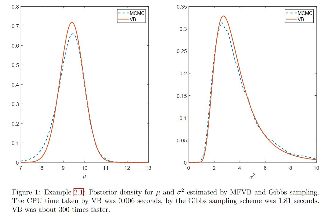
However, it’s often a better idea to initialize $\mu_q,\s_q^2$ as it is easier to guess the values related to location parameters than the scale parameters. Figure 1 plots the posterior densities estimated by the MFVB algorithm derived above, and by Gibbs sampling.

It is straightforward to extend the MFVB procedure in Algorithm 1 to the general case where $\theta$ is divided into $k$ blocks $\t=(\t_1^\top,\t_2^\top,…,\t_k^\top)^\top$, and where we want to approximate the posterior $p(\t_1,\t_2,…,\t_k|y)$ by $q(\t)=q_1(\t_1)q_2(\t_2)…q_k(\t_k)$.

The optimal $q_j(\t_j)$ that maximizes $\LB(q)$, when $q_1,…,q_{j-1},q_{j+1},…,q_{k}$ are fixed, is

\[\tag{9}\label{MFVB-9} q_j(\t_j)\propto \exp\big(\E_{-\t_j}[\log p(y,\t)]\big),\;\;\;j=1,...,k.\]

Here $\E_{-\t_j}(\cdot)$ denotes the expectation w.r.t. $q_1$,…, $q_{j-1}$, $q_{j+1}$,…, $q_{k}$, i.e.,

\[\E_{-\t_j}\big[\log p(y,\t)\big]:=\int q_1(\theta_1)...q_{j-1}(\theta_{j-1})q_{j+1}(\theta_{j+1})...q_{k}(\theta_k)\log p(y,\t)d\theta_1....d\theta_{j-1}d\theta_{j+1}...d\theta_k.\]

A similar procedure to Algorithm Algorithm 1 can be developed, in which we first initialize the parameters in the $k-1$ factors $q_1,…,q_{k-1}$, then update $q_k$ and the other factors recursively.

---

Example 3.1: Fixed From VB with control variates for Bayesian Linear Regression

Suppose that the VB approximation is $q_\l(\mu,\sigma^2)=q(\mu)q(\sigma^2)$ with $q(\mu)=\N(\mu_\mu,\sigma_\mu^2)$ and $q(\sigma^2)=\text{Inverse-Gamma}(\a_{\sigma^2},\b_{\sigma^2})$. This toy example is simply to demonstrate the use of Algorithm 4, we do not focus on the approximation accuracy here.

The model parameter is $\theta=(\mu,\sigma^2)^\top$ and the variational parameter $\lambda=(\mu_\mu,\sigma_\mu^2,\a_{\sigma^2},\b_{\sigma^2})^\top$. In order to implement Algorithm 4, we need $h_\lambda(\theta)=h(\theta)-\log q_\l(\t)$ with

\[\begin{eqnarray} h(\theta)&=&\log \big(p(\mu)p(\sigma^2)p(y\mid \mu,\sigma^2)\big)\\ &=&-\frac{n+1}{2}\log(2\pi)-\frac12\log(\sigma_0^2)-\frac{(\mu-\mu_0)^2}{2\sigma_0^2}+\alpha_0\log(\beta_0)-\log\Gamma(\a_0)-(\frac{n}{2}+\a_0+1)\log(\s^2)\\ &&\phantom{cccc}-\frac{\b_0}{\s^2}-\frac{1}{2\s^2}\sum_{i=1}^n(y_i-\mu)^2,\\ \log q_\l(\t)&=&\a_{\s^2}\log\b_{\s^2}-\log\Gamma(\a_{\s^2})-(\a_{\s^2}+1)\log\s^2-\frac{\b_{\s^2}}{\s^2}-\frac12\log(2\pi)-\frac12\log(\s_{\mu}^2)-\frac{(\mu-\mu_\mu)^2}{2\s_\mu^2}, \end{eqnarray}\]

and

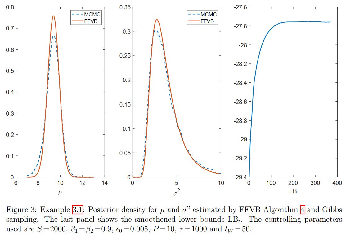
\[\nabla_\l\log q_\l(\t)=\Big(\frac{\mu-\mu_\mu}{\s_\mu^2},-\frac{1}{2\s_\mu^2}+\frac{(\mu-\mu_\mu)^2}{2\s_\mu^4},\log\b_{\s^2}-\frac{\Gamma'(\a_{\s^2})}{\Gamma(\a_{\s^2})}-\log\s^2,\frac{\a_{\s^2}}{\b_{\s^2}}-\frac{1}{\s^2} \Big)^\top.\]

We are now ready to implement Algorithm 4. Figure 3 plots the estimate of the posterior densities together with the lower bound. The Variational Bayes estimates appear to be quite close to the Gibbs sampling estimates in this example, with some small discrepancy between them. These estimates can be improved with more advanced variants of FFVB presented later.

---

Example 3.2: Fixed From VB with control variates and natural gradient for Bayesian Linear Regression

In order to implement Algorithm 5, apart from $h_\l(\t)$ and $\nabla_\l\log q_\l(\t)$ as in Example 3.1, we need the Fisher information matrix $I_F$. It can be seen that this is a diagonal block matrix with two main blocks

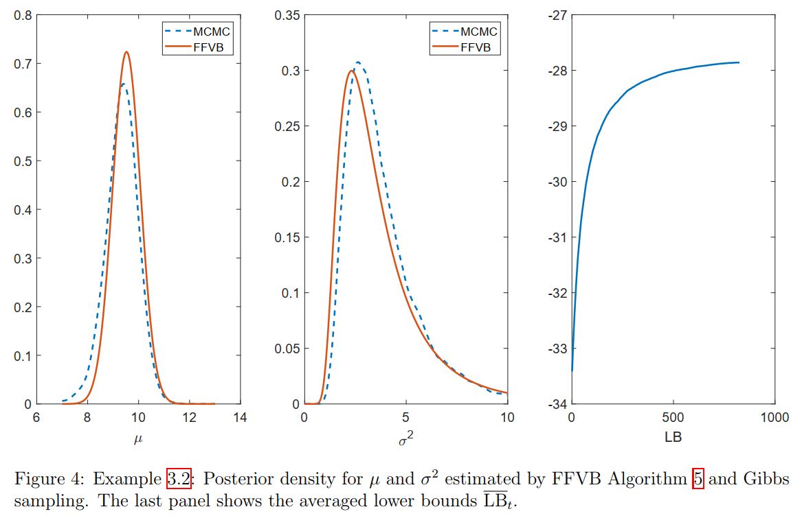
\[\begin{pmatrix}\frac{1}{\s_\mu^2}& 0\\ 0&\frac{1}{2\s_\mu^4} \end{pmatrix},\;\;\;\text{ and }\;\;\; \begin{pmatrix} \frac{\partial^2\log\Gamma(\a_{\s^2})}{\partial \a_{\s^2}\partial \a_{\s^2}}&-\frac{1}{\b_{\s^2}}\\ -\frac{1}{\b_{\s^2}} & \frac{\a_{\s^2}}{\b_{\s^2}^2} \end{pmatrix}.\]

Figure 4 shows the estimated densities together with the lower bound estimates. In this example, Algorithm \ref{algorithm 3} appears to produce a very similar approximation as in Algorithm \ref{algorithm 2}.

The choice of the variational distribution $q_\l(\mu,\sigma^2)=q(\mu)q(\sigma^2)$ in Examples 3.1 and Examples 3.2 ignores the posterior dependence between $\mu$ and $\sigma^2$. There are several alternatives that can improve this. One of these is to use Gaussian VB to approximate the posterior of the transformed parameter $\theta=\big(\mu,\log(\sigma^2)\big)$. Another alternative is presented in Examples 3.3 below.

---

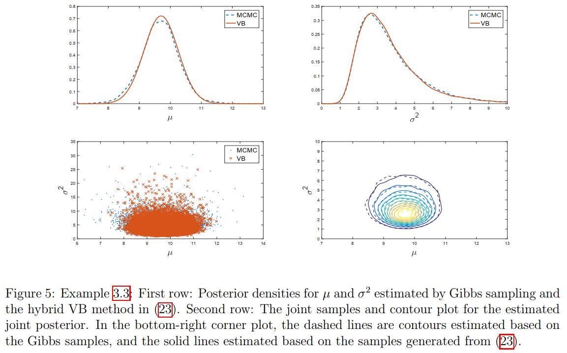
Example 3.3: Hybrid Fixed From VB for Bayesian Linear Regression

This distribution, as the joint distribution of $\mu$ and $\sigma^2$, doesn’t have a standard form, however, it is straightforward to sample from it. This variational distribution exploits the standard form of the full conditional $p(\sigma^2|y,\mu)$, which is inverse-Gamma, and takes into account the posterior dependence between $\mu$ and $\sigma^2$.

The variational parameter $\lambda$ now only consists of $\mu_\mu$ and $\sigma_\mu^2$. Using (16), the gradient of the lower bound is

\[\nabla_\lambda\LB(\lambda)=\E_{q_\lambda(\mu,\sigma^2)}\Big(\nabla_\lambda\log \wt q_\lambda(\mu)\times h_\lambda(\theta)\Big)\]

with

\[h_\lambda(\theta)=\log p(\mu,\sigma^2)+\log p(y|\mu,\sigma^2)-\log \wt q_\lambda(\mu)-\log p(\sigma^2|y,\mu).\]

Algorithm Algorithm 4 or Algorithm 5 now can be applied.

Figure 5 shows the estimated results. As shown, this ``hybrid’’ VB approximation is highly accurate in terms of both marginal density estimate and the joint density estimate.

---

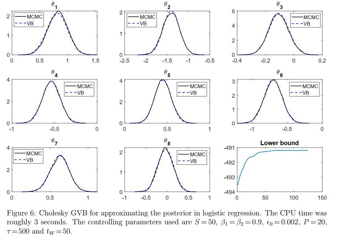
Example 3.4: Cholesky GVB for Bayesian Logistic Regression

To implement the Cholesky GVB method, all we need is the function

\[\tag{27}\label{eqn:h_function_ex4}h(\theta)=\log p(\theta)+\log p(y|X,\theta)=-\frac{d}{2}\log(2\pi)-\frac{d}{2}\log(\sigma_0^2)-\frac{\theta^\top\theta}{2\sigma_0^2}+y^\top X\theta-\sum_{i=1}^n\log\big(1+\exp(x_i^\top\theta)\big),\]

and its gradient

\[\tag{28}\label{eqn:grad_h_function_ex4_1}\nabla_\theta h(\theta)=-\frac{1}{\sigma_0^2}\theta+X^\top\big(y-\pi(\theta)\big)\]

with

\[\tag{29}\label{eqn:grad_h_function_ex4_2}\pi(\theta)=\Big(\frac{1}{1+\exp(-x_1^\top\theta)},\cdots,\frac{1}{1+\exp(-x_n^\top\theta)}\Big)^\top.\]

The Labour Force Participation dataset contains information of $753$ women with one binary variable indicating whether or not they are currently in the labour force together with seven covariates such as number of children under 6 years old, age, education level, etc. Figure 6 plots the VB approximation for each coefficient $\theta_i$ together with the lower bound estimates over the iterations.

---