CGVB for Logistic Regression model with AutoDiff Github code
This example implements the example 3.4 shown in the VB tutorial paper but we use Matlab AutoDiff to automatically compute the $\nabla_\theta h(\theta)$ term given a function to compute the $h(\theta)$ term. See Use Automatic Differentiation In Deep Learning Toolbox
Load the LabourForce data as a matrix. The last column is the response variable.
% Random seed to reproduce results
rng(2020)

% Load the LabourForce dataset
labour = readData('LabourForce',...
                  'Type','Matrix',...
                  'Intercept',true);
Prepare variables needed to run the VB algorithm and to define the custom model.
% Number of input features
n_features = size(labour,2)-1;
setting.Prior = [0,50];
In this example, we use the CGVB technique to fit the custom model on the labour data. To run the CGVB technique with the custom model, we need to specify the handle of the function defining the custom model as the first input argument. We also need to explicitly provide the number of model parameters for the 'NumParams' argument. Finally, we need to pass additional information, e.g. priors, stored in the struct setting to the 'Setting' argument. This setting variable then will be passed to the custom function as the input argument.
%% Run Cholesky GVB with random initialization
Post_CGVB_manual = CGVB(@grad_h_func_logistic,labour,...
                        'NumParams',n_features,... % Number of model parameters
                        'Setting',setting,...      % Additional setting of the custom models
                        'LearningRate',0.002,...   % Learning rate
                        'NumSample',50,...         % Number of samples to estimate gradient of lowerbound
                        'MaxPatience',20,...       % For Early stopping
                        'MaxIter',5000,...         % Maximum number of iterations
                        'MeanInit',theta_init ,... % Randomly initialize parameters using
                        'GradWeight1',0.9,...      % Momentum 1
                        'GradWeight2',0.9,...      % Momentum 2
                        'WindowSize',10,...        % Smoothing window for lowerbound
                        'GradientMax',10,...       % For gradient clipping
                        'LBPlot',true);
The output Post is a struct storing information about estimation results and the VB algorithm. In order to use Matlab AutoDiff to automatically evalulate the gradient of $h(\theta)$, we need to define a function to compute the $h(\theta)$ term using the mathematical derivation shown in the tutorial example 3.4.
%% We need to define a function to compute the h(theta) term
% Input:
%   data: 2D array
%   theta: Dx1 array
%   setting: struct
% Output:
%   h_func: h(theta) = log p(y|theta) + log p(theta)
function h_func = h_func_logistic(data,theta,setting)

    % Extract additional settings
    d = length(theta);
    sigma2 = setting.Prior(2);

    % Extract data
    y = data(:,end);
    X = data(:,1:end-1);

    % Compute log likelihood
    aux = X*theta;
    log_lik = y.*aux-log(1+exp(aux));
    log_lik = sum(log_lik);

    % Compute log prior
    log_prior =-d/2*log(2*pi)-d/2*log(sigma2)-theta'*theta/sigma2/2;

    % h = log p(y|theta) + log p(theta)
    h_func = log_lik + log_prior;

end
Next, we need to define a function contain the dlgradient() function to compute derivatives using automatic differentiation.
%% Function containing dlgradient to run AutoDiff for the h_func_logistic function
function [h_func_grad,h_func] = grad_h_func_logistic_AD(data,theta,setting)

    h_func = h_func_logistic(data,theta,setting);
    h_func_grad = dlgradient(h_func,theta);
end
Finally, we define the function grad_h_func_logistics to call the function containing the dlgradient() function using the dlfeval() function. We have to explicitly convert the model parameters from Matlab ordinary array to dlarray array data type. After obtain the $\nabla_\theta h(\theta)$ and $h(\theta)$ terms, we have to convert these two variables back to Matlab ordinary array using the extractdata() function.
%% Define function to compute gradient of h function for Logistic regression
% Input:
%   data: 2D array
%   theta: Dx1 array
%   setting: struct
% Output:
%   h_func: Scalar
%   h_func_grad: Dx1 array
function [h_func_grad,h_func] = grad_h_func_logistic(data,theta,setting)

    % Convert parameters to dlarray data type
    theta_AD = dlarray(theta);

    % Evaluate the function containing dlgradient using dlfeval
    [h_func_grad_AD,h_func_AD] = dlfeval(@grad_h_func_logistic_AD,data,theta_AD,setting);

    % Convert parameters from dlarray to matlab array
    h_func_grad = extractdata(h_func_grad_AD);
    h_func = extractdata(h_func_AD);

    % Make sure the output is a column vector
    h_func_grad = reshape(h_func_grad,length(h_func_grad),1);

end
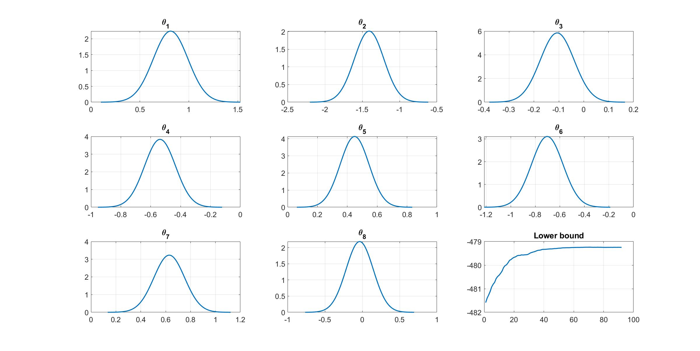
We can manually plot the variational distribution together with the lowerbound.
%% Plot variational distributions and lowerbound
figure
% Extract variation mean and variance
mu_vb     = Post_CGVB_manual.Post.mu;
sigma2_vb = Post_CGVB_manual.Post.sigma2;

% Plot the variational distribution for the first 8 parameters
for i=1:8
    subplot(3,3,i)
    vbayesPlot('Density',{'Normal',[mu_vb(i),sigma2_vb(i)]})
    grid on
    title(['\theta_',num2str(i)])
    set(gca,'FontSize',15)
end

% Plot the smoothed lower bound
subplot(3,3,9)
plot(Post_CGVB_manual.Post.LB_smooth,'LineWidth',2)
grid on
title('Lower bound')
set(gca,'FontSize',15)
The convergence of the lowerbound shows that the CGVB works properly in this example.