LogisticRegression class Github code
Create Logistic Regression model object
Syntax
Mdl = LogisticRegression(NumFeatures,Name,Value)
Description
mdl = LogisticRegression(NumFeatures,Name,Value) returns LogisticRegression model object Mdl given number of model parameters NumFeatures. Name and Value specify additional options using one or more name-value pair arguments. For example, users can specify different choices of priors for model parameters.
See: Input Arguments, Output Argument, Examples
Input Arguments
Data type: positive integer
Number of model parameters, which is also the number of data features or covariates or independent variables.
Name-Value Pair Arguments
Specify optional comma-separated pairs of Name,Value arguments. Name is the argument name and Value is the corresponding value. Name must appear inside quotes. You can specify several name and value pair arguments in any order as Name1,Value1,...,NameN,ValueN.
Example: 'Prior',{'Normal',[0,10]},'CutOff',0.6 specifies that the prior distribution of model parameters is a normal distribution with $0$ mean and $10$ variance, and the cutoff probability is $0.06$.
'Prior' - Prior distribution of model parameters
Data Type: Cell Array
Prior distribution of the model parameters, specified as the comma-separated pair consisting of 'Prior' and a cell array of distribution name and distribution parameters. Distribution parameters are specified as an array.
| Prior Name | Description |
|---|---|
'Normal' | Normal distribution $\mathcal{N}(\mu,\sigma^2)$ (default) |
'Gamma' | Gamma distribution $\Gamma(\alpha,\beta)$ |
'Inverse-Gamma' | Gamma distribution $\Gamma^{-1}(\alpha,\beta)$ |
Default: {'Normal',[0,1]}
Example: 'Prior',{'Normal',[0,10]}
Output Arguments
Data type: LogisticRegression Object
LogisticRegression is an object of the LogisticRegression class with pre-defined properties and functions.
Object Properties
The LogisticRegression object properties include information about model-specific information, coefficient estimates and fitting method.
| Properties | Data type | Description{: .text-center} |
|---|---|---|
ModelName | string (r) | Name of the model, which is 'LogisticRegression' |
NumParams | integer (+) | Number of model parameters |
Cutoff | float | Cut-off probabitlity |
Post * | struct | Information about the fittedd method used to estimate model paramters |
Coefficient * | cell array (r) | • Estimated Mean of model parameters • Used to doing point estimation for new test data |
CoefficientVar * | cell array (r) | Variance of coefficient estimates |
LogLikelihood * | double (r) | Loglikelihood of the fitted model. |
FittedValue * | array (r) | Fitted probability |
Notation:
- * $\rightarrow$ object properties which are only available when the model is fitted. Default value is
None. - (+) $\rightarrow$ positive number.
- (r) $\rightarrow$ read-only properties.
Object Methods
Use the object methods to initialize model parameters, predict responses, and to visualize the prediction.
| vbayesInit | Initialization method of model parameters |
| vbayesPredict | Predict responses of fitted DeepGLM models |
Examples
Fit a LogisticRegression model for binary response Github code
Fit a LogisticRegression model to LabourForce data using CGVB
Load the LabourForce data using the readData() function. The data is a matrix with the last column being the response variable. Set the 'Intercept' argument to be true to add a column of 1 to the data matrix as intercepts.
% Load the LabourForce dataset
labour = readData('LabourForce',...    % Dataset name
                  'Type','Matrix',...  % Store data as a 2D array (default)
                  'Intercept',true);   % Add column of intercept (default)
Create a LogisticRegression model object by specifying the number of parameters as the input argument. Change the variance of the normal prior to $10$.
% Number of input features
n_features = size(labour,2)-1;
% Define a LogisticRegression model object
Mdl = LogisticRegression(n_features,...
                         'Prior',{'Normal',[0,10]});
Run CGVB to obtain VB approximation of the posterior distribution of model parameters.
%% Run Cholesky GVB with random initialization
Post_CGVB = CGVB(Mdl,labour,...
                'LearningRate',0.002,...  % Learning rate
                'NumSample',50,...        % Number of samples to estimate gradient of lowerbound
                'MaxPatience',20,...      % For Early stopping
                'MaxIter',5000,...        % Maximum number of iterations
                'GradWeight1',0.9,...     % Momentum weight 1
                'GradWeight2',0.9,...     % Momentum weight 2
                'WindowSize',10,...       % Smoothing window for lowerbound
                'StepAdaptive',500,...    % For adaptive learning rate
                'GradientMax',10,...      % For gradient clipping
                'LBPlot',false);          % Dont plot the lowerbound when finish
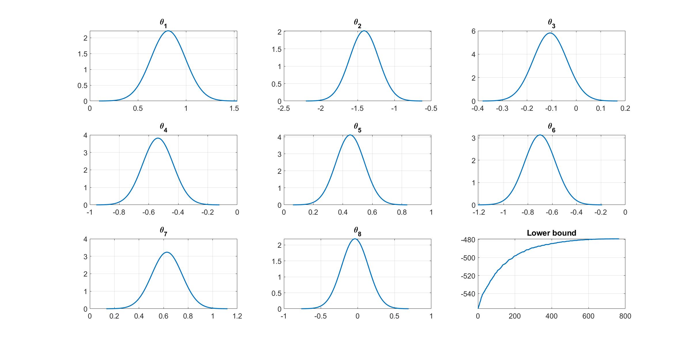
Given the estimation results, we can plot the variational distribution together with the lowerbound to check the performance of the CGVB algorithm.
% Plot variational distributions and lowerbound
figure
% Extract variation mean and variance
mu_vb     = Post_CGVB.Post.mu;
sigma2_vb = Post_CGVB.Post.sigma2;

% Plot the variational distribution for the first 8 parameters
for i=1:n_features
    subplot(3,3,i)
    vbayesPlot('Density',{'Normal',[mu_vb(i),sigma2_vb(i)]})
    grid on
    title(['\theta_',num2str(i)])
    set(gca,'FontSize',15)
end

% Plot the smoothed lower bound
subplot(3,3,9)
plot(Post_CGVB.Post.LB_smooth,'LineWidth',2)
grid on
title('Lower bound')
set(gca,'FontSize',15)
The plot of lowerbound shows that the CGVB algorithm works properly.
Reference
[1] Tran, M.-N., Nguyen, T.-N., Nott, D., and Kohn, R. (2020). Bayesian deep net GLM and GLMM. Journal of Computational and Graphical Statistics, 29(1):97-113. Read the paper
See Also
DeepGLM $\mid$ rech $\mid$ Custom model $\mid$ CGVB