Define a VAR(1) model as a function handle Github code
This example shows how to define a VAR(1) model as a function handle to work with VBLab supported VB algorithms.
Let ${y_t,\ t=1,2,…}$ be a $m$-dimensional time series. Consider the vector autoregressive model of order 1, denoted as VAR(1), defined as:
\[y_t = c+ Ay_{t-1} + u_t, \quad u_t \sim^{iid} \mathcal{N}(0,\Gamma)\]where $c$ is a $m$-vector and $A$ a $(m\times m)$-matrix of regression coefficients. For the simplicity, let’s assume $\Gamma$ is known. The vector of model parameters is $\theta=(c^\top,\text{vec}(A)^\top)^\top$. Suppose that the prior is $p(\theta) = \mathcal{N}(0,\sigma_0^2I_d)$ with $I_d$ the identity matrix and $d=m(m+1)$.
Then the $h(\theta)$ term of the VAR(1) model can be derived as
\[\begin{eqnarray}\tag{1}\label{eqn:var1-1} h(\theta)&=&\log p(\theta)+\log p(y|\theta)\\ &=&-\frac{d}{2}\log(2\pi)-\frac{d}{2}\log(\sigma_0^2)-\frac{\theta^\top\theta}{2\sigma_0^2}-\frac{m(T-1)}{2}\log(2\pi)-\frac{T-1}{2}\log|\Gamma|\\ &-&\frac{1}{2} \sum_{t=2}^{T} \left((y_t-Ay_{t-1}-c)^\top \Gamma^{-1} (y_t-A y_{t-1}-c)\right). \end{eqnarray}\]and the $\nabla_\theta h(\theta)$ term can be written as
\[\begin{eqnarray}\tag{2}\label{eqn:var1-2} \nabla_\theta h(\theta) = \begin{pmatrix} \nabla_c h(\theta)\\ \nabla_{\text{vec}(A)}h(\theta) \end{pmatrix} \end{eqnarray}\]with
\[\tag{3}\label{eqn:var1-3}\nabla_c h(\theta) = -\frac{1}{\sigma_0^2}c+\Gamma^{-1}\big(\sum_{t=2}^T (y_t-A y_{t-1}-c)\big)\]and
\[\tag{4}\label{eqn:var1-4}\nabla_{\text{vec}(A)}h(\theta) = -\frac{1}{\sigma_0^2}\vec(A)+\sum_{t=2}^T y_{t-1}\otimes \big(\Gamma^{-1} (y_t-A y_{t-1}-c)\big).\]Given the equations to compute the $h(\theta)$ and $\nabla_\theta h(\theta)$, we will define a function, following the template discussed before, to define the VAR(1) model that can work with VBLab supported VB algorithms.
For demonstration, we create a simulation data including $2$ series of $100$ observations, generated from a uniform distribution.
% Setting
m = 2;   % Number of time series
T = 100; % Number of observations

% Generate data
y = randn(m,T);
Then, we prepare the additional information needed to compute the $h(\theta)$ and $\nabla_\theta h(\theta)$ terms of the VAR(1) model. This information will be stored in a struct named setting. The additional information include priors, number of model parameters, indexes of model parameters in the vector of variational mean and the covariance matrix $\Gamma$.
% Additional setting
setting.prior.mu = 0;
setting.prior.var = 1;
setting.y.mu = 0;
setting.idx.c = 1:m;          % Indexes to extract c from a vector of all parameters
setting.idx.A = m+1:m+m^2;    % Indexes to extract A from a vector of all parameters
setting.num_params = m + m^2; % Number of model parameters
setting.Gamma = 0.1*eye(m);   % Fixed covariance matrix
Next we prepare initial values for the variantional mean (optional) and run the CGVB algorithm to estimate the model parameters
% Prepare theta
c = rand(m,1);
A = rand(m);

% Initial variational mean
theta = [c;A(:)];

Post_CGVB_VAR = CGVB(@grad_h_theta_VAR1,y,...
                     'NumParams',setting.num_params,...
                     'Setting',setting,...
                     'LearningRate',0.002,...       % Learning rate
                     'NumSample',50,...             % Number of samples to estimate gradient of lowerbound
                     'MaxPatience',20,...           % For Early stopping
                     'MaxIter',5000,...             % Maximum number of iterations
                     'GradWeight1',0.9,...          % Momentum 1
                     'GradWeight2',0.9,...          % Momentum 2
                     'WindowSize',10,...            % Smoothing window for lowerbound
                     'GradientMax',10,...           % For gradient clipping
                     'LBPlot',false);
Finally, we need to define the function grad_h_theta_VAR1 using the template discussed in how to define models as function handles. The grad_h_theta_VAR1 can be defined in a seperate script named grad_h_theta_VAR1 or at the end of the example script.
%% Function to compute the gradient of h(theta) and h(theta). This can be defined in a separate file
% Input:
%       y: mxT matrix with M number of time series and T lenght of each time series
%       theta: Dx1 array of model parameters
%       setting: struct of additional information to compute gradient h(theta)
% Output:
%       grad_h_theta: Dx1 array of gradient of h(theta)
%       h_theta: h(theta) is scalar
function [grad_h_theta,h_theta] = grad_h_func_VAR1(y,theta,setting)

    % Extract size of data
    [m,T] = size(y);

    % Extract model settings
    prior_params = setting.Prior;
    d = setting.num_params;
    idx = setting.idx;
    Gamma = setting.Gamma;
    Gamma_inv = Gamma^(-1);

   % Extract params from theta
    c = theta(idx.c);                               % c is a Dx1 colum
    A = reshape(theta(idx.A),length(c),length(c));  % A is a DxD matrix

    % Log prior
    log_prior = Normal.logPdfFnc(theta,prior_params);

    % Log likelihood
    log_llh = 0;
    for t=2:T
        log_llh = log_llh -0.5*(y(:,t) - A*y(:,t-1)-c)' * Gamma_inv * (y(:,t) - A*y(:,t-1)-c);
    end
    log_llh = log_llh - 0.5*m*(T-1)*log(2*pi) - 0.5*(T-1)*log(det(Gamma));

    % h(theta)
    h_theta = log_prior + log_llh;

    % Gradient of log prior
    grad_log_prior = Normal.GradlogPdfFnc(theta,prior_params);

    % Gradient of log likelihood;
    grad_llh_c = 0;
    grad_llh_A = 0;
    for t=2:T
        grad_llh_c = grad_llh_c + Gamma_inv*(y(:,t) - A*y(:,t-1)-c);
        grad_llh_A = grad_llh_A + kron(y(:,t-1),Gamma_inv*(y(:,t) - A*y(:,t-1)-c));
    end

    grad_llh = [grad_llh_c;grad_llh_A(:)];

    % Gradient h(theta)
    grad_h_theta = grad_log_prior + grad_llh;

    % Make sure grad_h_theta is a column
    grad_h_theta = reshape(grad_h_theta,d,1);

end
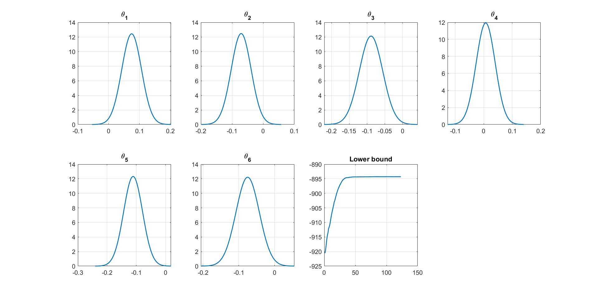
We can manually plot the variational distribution together with the lowerbound. The convergence of the lowerbound shows that the CGVB works properly in this example.
% Plot varitional distribution and of model parameters
figure
% Extract variation mean and variance
mu_vb     = Post_CGVB_VAR.Post.mu;
sigma2_vb = Post_CGVB_VAR.Post.sigma2;

% Plot the variational distribution of each parameter
for i=1:mdl.num_params
    subplot(2,4,i)
    vbayesPlot('Density',...
               'Distribution',{'Normal',[mu_vb(i),sigma2_vb(i)]})
    grid on
    title(['\theta_',num2str(i)])
    set(gca,'FontSize',15)
end

% Plot the smoothed lower bound
subplot(2,4,7)
plot(Post_CGVB_VAR.Post.LB_smooth,'LineWidth',2)
grid on
title('Lower bound')
set(gca,'FontSize',15)