VAFC
Fit VBLab supported or custom models using the VAFC method
Syntax
Post = VAFC(Mdl,data,Name,Value)
Description
Post = VAFC(Mdl,data,Name,Value) runs the VAFC algorithm to return the estimation results Post given the model Mdl and data data. The model Mdl can be a VBLab supported or custom model. The custom models can be defined as class objects or function handles. Name and Value specify additional options using one or more name-value pair arguments. For example, you can specify how many samples used to estimate the lower bound.
See: Input Arguments, Output Argument, Examples
Input Arguments
Data type: VBLab model object | custome model object | function handle
The statistical models containing unknown parameters, can be specified as:
Data type: 2D array | 1D array | table
The data to which the model Mdl is fit, specified as a table or dataset array.
For cross-sectional data, VAFC takes the last variable as the response variable and the others as the predictor variables.
For time series data, the data can be stored in a row or column 1D array.
Name-Value Pair Arguments
Specify optional comma-separated pairs of Name,Value arguments. Name is the argument name and Value is the corresponding value. Name must appear inside quotes. You can specify several name and value pair arguments in any order as Name1,Value1,...,NameN,ValueN.
Example: 'LearningRate',0.001,'LBPlot',true specifies that the learning rate of the VAFC algorithm is set to be $0.001$ and the plot of the covergence of the lowerbound is shown at the end of the algorithm.
| Name | Default Value | Notation | Description |
|---|---|---|---|
'GradWeight' | 0.9 | Adaptive learning weight | |
'GradientMax' | 10 | $\ell_\text{threshold}$ | Gradient clipping threshold |
'InitValue' | None | Initial values of varitional mean | |
'LBPlot' | true | Flag to plot the lowerbound or not | |
'LearningRate' | 0.01 | $\epsilon_0$ | Fixed learning rate |
'MaxIter' | 1000 | Maximum number of iterations | |
'MaxPatience' | 20 | $P$ | Maximum patience for early stopping |
'NumFactor' | 4 | $f$ | Number of factors of the factor loading matrix |
'NumSample' | 50 | $S$ | Monte Carlo samples to estimate the lowerbound |
'NumParams' | None | Number of model parameters | |
'SaveParams' | false | Flag to save training parameters or not | |
'Setting' | None | Additional setting for custom models | |
'SigInitScale' | 0.1 | Constant factor for initialization | |
'StdForInit' | 0.01 | Standard deviation of normal distribution for initialization | |
'StepAdaptive' | 'MaxIter'/2 | $\tau$ | Threshold to start reducing learning rates |
'TrainingLoss' | PPS | Training loss over VB iterations | |
'Validation' | 0.1 | Subset of training data used for validation | |
'ValidationLoss' | PPS | Validation loss over VB iterations | |
'Verbose' | true | Flag to show real-time fitting information or not | |
'WindowSize' | 50 | Rolling window size to smooth the lowerbound |
'GradWeight' - Adaptive learning weight 1
Data Type: Double
The adaptive learning rate.
Must be a number between $0$ and $1$.
Default: 0.9
Example: 'GradWeight',0.95
'GradientMax' - Gradient clipping threshold
Data Type: Double | Positive
The maximum value to prevent the exploding gradient problem that occurs when the gradient gets too large, thus making the optimization for the model parameters (e.g., using gradient descent) highly unstable.
Default: 100
Example: 'GradientMax',10
'InitValue' - Initial value of varitional mean
Data Type: Column vector
The column vector of initial values of variational parameters. For example, we can use the point estimation of model parameters from MLE to initialize the VB techniques.
Default: None
Example: 'InitValue',zeros(D,1)
'LBPlot' - Flag to plot the lowerbound or not
Data Type: True | False
Flag to plot the smoothed lowerbound over iterations to quicly check the convergence of the VB algorithm.
Default: true
Example: 'LBPlot',false
'LearningRate' - Fixed learning rate
Data Type: Double | Between 0 and 1
The fixed learning rate $\epsilon_0$ to update the variational parameters in each VB iteration in Algorithm 7.
Must be a number between $0$ and $1$.
Default: 0.01
Example: 'LearningRate',0.001
'MaxIter' - Maximum number of iterations
Data Type: Integer | Positive
Maximum number of VB iterations for early stopping. If the 'BatchSize' argument is specified, users have to use the 'MaxEpoch' argument to specify the maximum number of iterations instead.
Default: 1000
Example: 'MaxIter',1000
'MaxPatience' - Maximum patience for early stopping
Data Type: Integer | Positive
Number of consecutive times that the validation loss, or lowerbound, is allowed to be larger than or equal to the previously smallest loss, or lowerbound, before the training is stopped, used as an early stopping criterion. This is denoted as $P$ in the VAFC section Default: 20
Example: 'MaxPatience',100
'NumFactor' - Number of factors
Data Type: Integer | Positive
Number of factors (columns) of the factor loading matrix discussion in the VAFC section
Default: 4
Example: 'NumFactor',10
'NumSample' - Monte Carlo samples to estimate the lowerbound
Data Type: Integer | Positive
Number of Monte Carlo samples needed to estimate the gradient of the lower bound. This is denoted as $S$ in the VAFC section
Default: 50
Example: 'NumSample',100
'NumParams' - Number of model parameters
Data Type: Integer | Positive
Number of model parameters.
- If the handle of the function calculating the $h(\theta)$ and $\nabla_\theta h(\theta)$ terms is provided, users have to specify a value for this argument.
- If a model object is specified, users have to set the number of parameters using the
NumParamsproperty of the model class. See how to define a custom model as a Maltab class object.
Default: None
Example: 'NumParams',{'Normal',[0,10]}
'SaveParams' - Flag to save training parameters or not
Data Type: true | false
Flag to save variational parameters in each VB iteration.
Default: false
Example: 'SaveParams',true
'Setting' - Additional setting for custom models
Data Type: struct
Additional settings that could be use to define custom models as function handlers.
The most efficient way is to define these additional setting as a struct. This struct then will be passed to the function handlers as an input. See how to define custom model as function handler.
Default: None
Example: 'Setting',prior with prior is a struct whose fields are prior distribution name and parameters, e.g. prior.name = 'Normal' and prior.params = [0,1].
'SigInitScale' - Constant factor for initialization
Data Type: double
The constant factor $c$ to scale the initial values.
Default: 0.1
Example: 'SigInitScale',0.5
'StdForInit' - Standard deviation of normal distribution for initialization
Data Type: double
The constant factor $\sigma$ to scale the convariance matrix of the normal distribution used to initialize the variational mean.
Only specify this argument when the argument 'InitMethod' is set to 'Random'.
Default: 0.01
Example: 'StdForInit',0.04
'StepAdaptive' - Threshold to start reducing learning rates
Data Type: Integer | Positive
The iteration to start reducing learning rate, which is denoted as $\tau$ in the VAFC section
By default, this is set as 'MaxIter'/2 or 'MaxEpoch'/2.
Must be smaller than 'MaxIter' or 'MaxEpoch'.
Default: 'MaxIter'/2 or 'MaxEpoch'/2
Example: 'StepAdaptive',300
'TrainingLoss' - Training loss over VB iterations
Data Type: string | cell array of strings
The VB algorithm uses lowerbound to access the convergence of the training phase.
However, users can also calculate the predictive scores evaluated on the training data over VB iterations. Users can specify a single metric, defined as a string, or multiple metrics, defined as a cell array of strings.
Available score metrics:
| PPS | Partial Predictive Score |
| MSE | Mean Squared Errors (for continuos output) |
| MAE | Mean Absoluted Errors (for continuos output) |
| CR | Classification rate (for binary output) |
For the PPS:
- If the models are specified as function handlers, users have to also specify function handlers to the argument
'LogLikFunc'to compute the log-likelihood of the custom models. - If the models are specified as class objects, users have to define a method named
logLik()to compute the log-likelihood of the custom models.
Default: None
Example: 'TrainingLoss',{'PPS','MSE'}
'Validation' - Subset of training data used for validation
Data Type: double between 0 and 1 | Integer
Number of observations of training data are used as validation data. The number of observations can be specified as a percentage (a number between 0 and 1) of training data or an integer smaller than the number of training observations.
Note: This option is only available for cross-sectional (tabular) data.
Default: None
Example: 'Prior',0.1 or 'Prior',1000
'ValidationLoss' - Validation loss computed during fitting phase
Data Type: string | cell array of strings
Calculate the predictive scores evaluated on the validation data over VB iterations. Users can specify a single metric, defined as a string, or multiple metrics, defined as a cell array of strings.
Available score metrics:
| PPS | Partial Predictive Score |
| MSE | Mean Squared Errors (for continuos output) |
| MAE | Mean Absoluted Errors (for continuos output) |
| CR | Classification rate (for binary output) |
For the PPS:
- If the models are specified as function handlers, users have to also specify function handlers to the argument
'LogLikFunc'to compute the log-likelihood of the custom models. - If the models are specified as class objects, users have to define a method named
logLik()to compute the log-likelihood of the custom models.
Note: This option is only available for cross-sectional (tabular) data.
Default: None
Example: 'ValidationLoss','MSE'
'Verbose' - Flag to show real-time fitting information or not
Data Type: True | False
By default, the index of the current iteration and lowerbound are shown in every iteration. Set 'Verbose' to be false to turn off these messages.
Default: true
Example: 'Verbose',false
'WindowSize' - Rolling window size to smooth the lowerbound
Data Type: Integer | Positive
Size of moving average window that used to smooth the lowerbound. Denoted as $t_W$ in Algorithm 7.
Default: 50
Example: 'WindowSize',100
Output Arguments
Data type: struct
Estimation results, specified as a structure with these fields:
| LB | Estimation of the Lower Bound over iterations |
| LB_smooth | Smoothed Lower Bound over iterations |
| lambda | Estimation of variational parameters |
| mu | Estimation of variational mean |
| B | The factor loading matrix component of the variational covariance matrix |
| C | The diagonal matrix component of the variational covariance matrix |
| Sigma | Estimation of the variational covariance matrix |
| sigma2 | Diagonal of the variational covariance matrix |
Examples Github code
This example shows how to use VAFC to fit a logistic regression model on the GermanCredit dataset. First, Load the GermantCredit data as a matrix. The last column is the response variable.
% Random seed to reproduce results
rng(2020)

% Load GermanCredit data.
credit = readData('GermanCredit',...    % Dataset name
                  'Type','Matrix',...   % Store data as a 2D array (default)
                  'Intercept', true);   % Add column of intercept (default)
Create a LogisticRegression model object by specifying the number of parameters as the input argument. We use the default priors which are standard normal distribution.
% Compute number of features
n_features = size(credit,2)-1;

% Create a Logistic Regression model object
Mdl = LogisticRegression(n_features);
Run VAFC to obtain VB approximation of the posterior distribution of model parameters. We use $10$ factors for the loading matrix of the variational covariance matrix.
%% Run VAFC with random initialization
Post_VAFC = VAFC(Mdl,credit,...
                 'NumFactor',10, ...      % Number of factors of the loading matrix
                 'NumSample',50,...       % Number of samples to estimate gradient of lowerbound
                 'LearningRate',0.05,...  % Learning rate
                 'MaxPatience',20,...     % For Early stopping
                 'MaxIter',10000,...      % Maximum number of iterations
                 'GradientMax',200,...    % For gradient clipping
                 'WindowSize',5, ...      % Smoothing window for lowerbound
                 'LBPlot',false);         % Dont plot the lowerbound when finish
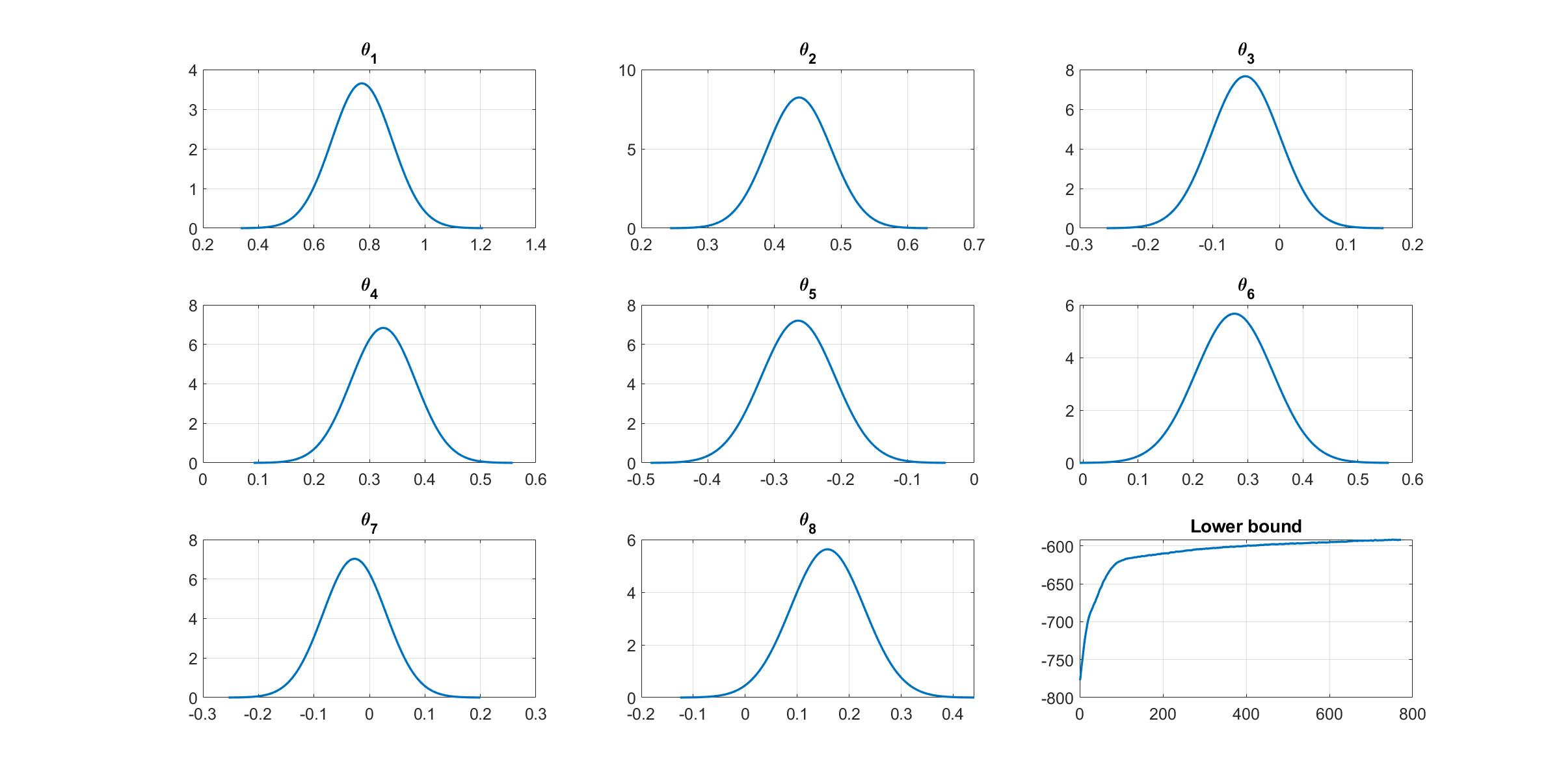
Given the estimation results, we can plot the variational distribution together with the lowerbound to check the performance of the VAFC algorithm.
%% Plot variational distributions and lowerbound
figure
% Extract variation mean and variance
mu_vb     = Post_VAFC.Post.mu;
sigma2_vb = Post_VAFC.Post.sigma2;

% Plot the variational distribution for the first 8 parameters
for i=1:8
    subplot(3,3,i)
    vbayesPlot('Density',{'Normal',[mu_vb(i),sigma2_vb(i)]})
    grid on
    title(['\theta_',num2str(i)])
    set(gca,'FontSize',15)
end

% Plot the smoothed lower bound
subplot(3,3,9)
plot(Post_VAFC.Post.LB_smooth,'LineWidth',2)
grid on
title('Lower bound')
set(gca,'FontSize',15)
The plot of lowerbound shows that the VAFC algorithm works properly.
Reference
[1] Ong, V. M.-H., Nott, D. J., and Smith, M. S. (2018). Gaussian variational approximation with a factor covariance structure. Journal of Computational and Graphical Statistics, 27(3):465-478. Read the paper
See Also
CGVB $\mid$ NAGVAC $\mid$ MGVB